Big Data and Data Analysis with Python
Nemanja Grubor
9 Jun 2021
•
12 min read
Introduction
In this article, we will talk about Big Data and Data Analysis with Python.
Due to the huge number of devices and users connected to the Internet, the amount of data is increasing at an exponential rate. Those companies that implement big data systems will have a significant competitive advantage in the market. This advantage primarily stems from the ability of entities to successfully make short-term and long-term decisions based on data that the system successfully analyzes and processes, and ultimately presents well into a meaningful whole.
Implementing a big data system is not easy, it requires significant long-term financial investments. The obstacles that a company encounters in implementing a big data system are not only financial but also human and technical.
One of the most popular programming languages in various components of a big data system is Python. The flexibility and power of Python are perhaps most visible in data analysis and processing.
Big Data### Definition of Big Data
The big data phenomenon is characterized by 3 Vs:
- Volume (large amounts of data)
- Velocity (continuous collection of new and digitalization of old data)
- Variety (different types and formats of data, including databases, documents, images, files, etc.)
The phenomenon of big data has almost only one role, and that is a timely and accurate information as a basis for quality assessments in business. The big data phenomenon is often placed in the context of artificial intelligence. Such characterization is often confusing. The phenomenon of big data doesn't revolve around the fact that a device or system learns to think or behave like a human by applying machine learning methods, but by applying mathematical, statistical, and computer methods to large data sets to obtain as accurate probabilities as possible in the decision-making process, e.g. the probability that a program contains malicious code or that we create the best possible prediction for its future behavior based on the consumer's purchase history.
Difference between big and small data
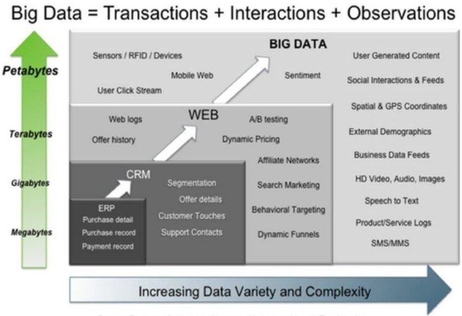
We can't consider large amounts of data to be small data that have mutated over time in terms of data size so that it can't be opened in traditional data processing programs (such as Excel), or in the database that exceeds the resources on the server on which it is stored. Such misperception is common among experts who believe that the application of existing knowledge and methods can analyze more complex and larger data sets, which can later lead to sudden financial costs and poor outcomes due to wrong decisions. In this context, the fundamental difference between so-called large and small data is best seen on the following image, which, on the Y-axis shows the amount of data generated by smaller systems, and on the X-axis the data diversity and complexity achieved by systems in larger categories:
Basic differences between big and small data are manifested in the:
- context of the aim to be achieved. Small data are usually designed to answer specific business questions. On the other hand, big data are designed with the goal of long-term use and time flexibility.
- location context. Small data are usually located within one institution, that is, on one server, and sometimes, just in one file. On the other hand, big data is dispersed on multiple Internet servers and across multiple institutions.
- context of structure and content. Small data are usually significantly structured, i.e. they come from one discipline or sector, which means that their structure is usually uniform. Big data, on the other hand, is not structured, i.e. data comes from multiple sources in various data structures and formats.
- context of data preparation. When it comes to small data, in most cases, the user prepares his own data which he usually uses for personal needs. With big data, data comes from multiple sources and multiple users.
- data lifetime context. The lifespan of small data is usually reduced to the lifetime of the project itself. With big data, data storage must be long-term, because their use is multifunctional and for future research, it is necessary to have previous data.
- context of financial investments. With small data, financial costs are limited, and users can recover from data loss relatively quickly. When applying the big data concept, data loss or unforeseen disaster can lead to the bankruptcy of the entity and significant financial losses.
- context of analysis. Small data is analyzed relatively easily and quickly, usually in one step and using a single procedure. For big data, with a few exceptions, data analysis usually takes steps in multiple steps. Data needs to be stored, prepared for processing, checked, analyzed, and interpreted.
Big Data and Python
Python as a Language for Data Analysis
In computer engineering, one of the most important things is the ability for computer algorithms to solve given problems quickly and efficiently, but also that their implementation is as simple and cheap as possible. It is natural to strive for optimized computer code or programming language that least burdens computer resources and provides a high degree of reliability. In certain situations, the use of such programming languages, e.g. C, Fortran, or ADA is inevitable to obtain maximum efficiency and effectiveness of the resources used in combination with high system reliability at critical moments.
But, it is not always wise to use such programming languages for a large number of the other tasks that can be done by other programming languages with much fewer lines of code, which is not always the case in modern enterprises.
It is necessary to consider the development time required to solve a particular problem in a programming language, the use of low-level programming languages in solving problems that don't need extremely high reliability and efficiency.
This is where high-level programming languages come to mind, that have a simpler syntax, flexibility, and easier maintenance system. This significantly shortens the time spent in the development or solution of a particular problem.
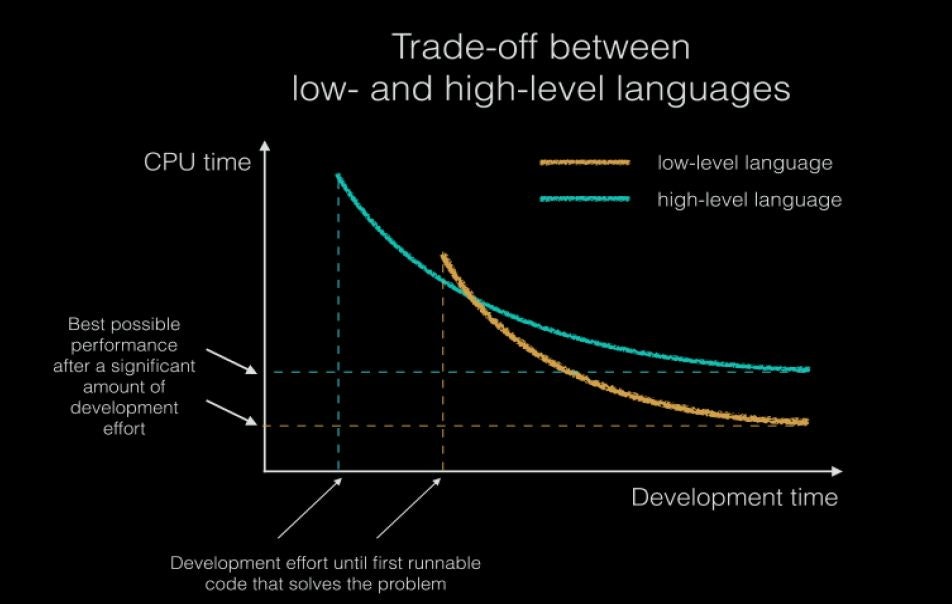
The above graph shows use the difference, i.e. the compromise between high-level and low-level programming languages. High-level programming languages have become extremely popular even in areas where significant savings in computer resources were previously required, primarily because the processing power measured in MIPS/$ (Millions of Instructions Per Second) has become cheaper. Due to the more competitive market of processor manufacturers, and human knowledge, i.e. human capital has become more expensive per hour of work due to the exponential growth of the Internet.
In many cases, the solution is seen in the use of multilingual programming models, where low-level programming languages are used for certain tasks that require a high level of reliability, and high-level programming languages for other parts. In this type of integration, programming languages such as Python, which has become synonymous with the so-called programming language that serves as a glue that combines time-critical and computationally intensive tasks with a simple user interface.
From this assumption, the modern Python has been developed, which became much more than the stated role of a stapler. In recent years, the entire ecosystem of accompanying development environments and libraries has been developed and came to life. Many of these "below the surface" libraries are written in a low-level language for best performance, while their control is maximally simplified by using simple and clear Python syntax. It is this ecosystem and the above facts, that are the reasons for the success of Python, which has become one of the most popular programming languages today.
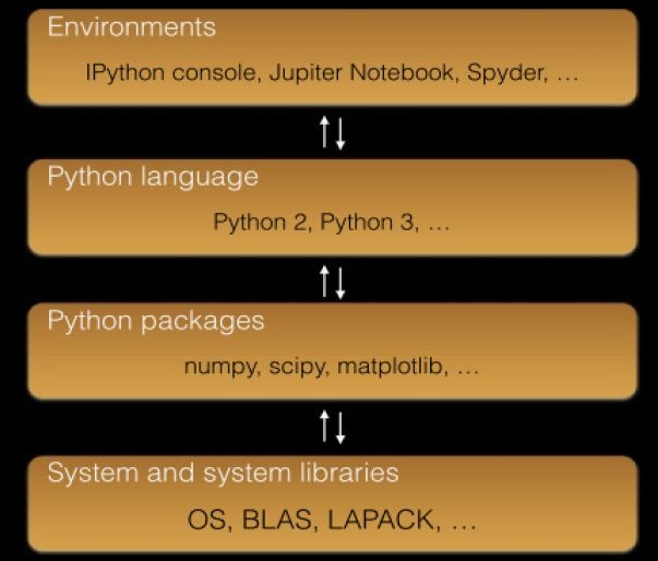
The above image best illustrates Python's ecosystem, where at the top of the chain are development environments in which a very simple and clear Python programming language syntax is written, and at the bottom of the chain are system libraries written in low-level programming languages that interact directly with the operating system. It is worth mentioning that the important fact that most development environments and software libraries are open-source, i.e. they come with free intellectual property licenses, which for the development of the developer of the application represents significant savings in the segment of development.
Popular Libraries for Data Analysis in Python
Pandas and Matplotlib Libraries
The Pandas library is one of the most well-known open-source libraries for data processing and manipulation. This library provides data structure processing that allows you to work with a variety of data types and time series in a fast and flexible way.
This library is designed for the following types of data:
- Spreadsheet data like Excel and SQL structured tables
- Sorted and unsorted time series of data
- Heterogeneous and homogeneous matrix data from different data structures
This library is suitable for the following types of operations:
- Easily processing missing data in a particular data set
- Data manipulation operations: columns can be inserted and deleted from the data frame
- Easily convert data from one data structure to another
- Smart data cutting and indexing
- Merging datasets
- Special functions for time series of data allow easy data analysis and processing on time series
The data processed with the help of the Pandas library are most often graphically displayed by the Matplotlib library, which is also the most popular library for graphical display. The biggest advantage of this library lies in its versatility, universality, and ease of use.
SciPy Library
This library is used for certain descriptive statistics and correlation functions.
The SciPy library is suitable for the following types of operations:
- Linear algebra
- Signal processing
- Fourier transforms
- Mathematical interpolation
- Statistics
- Multidimensional image processing
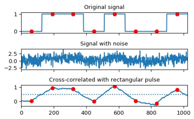
In the image below, we can see one of the examples of using the SciPy library when processing signals.
We will also see the Scikit-learn library in linear regression later, although this library is most common in machine learning.
Practical Examples of Data Analysis in Python
Descriptive Statistics in Python
Descriptive statistics is a part of mathematical statistics used to describe and better understand measured (or given) sets of data, i.e. descriptive statistics describes data through numerical summarization, tables, and graphs. The basic concepts of descriptive statistics are:
- Sum of data
- Largest and smallest data
- Range - the difference between the largest and smallest data
- Arithmetic mean (average)
- Median - half of the data is above and half below the median
- The first quartile (lower quartile) - a number of which is less than or equal to 25% of the data
- The second quartile - a number of which is less than or equal to 50% of the data. The second quartile is the same as the median.
- The third quartile (upper quartile) - a number of which is less than or equal to 75% of the data
- Sample mode - the data that appears most often in the sample
- Feature variation range
- Variance and standard deviation
- Variation coefficient
For statistical processing example, we will use the following Python libraries:
- SciPy
- Numpy
- Pandas
import numpy as np
import pandas as pd
from pandas import Series, DataFrame
import scipy
from scipy import stats
assoc = pd.read_excel("associations.xlsx")
assoc.columns = ['groupby_col', 'year', 'amount']
assoc.head()
# Sum of data
assoc.groupby(['groupby_col'])[['amount']].sum()
# Median
assoc.groupby(['year'])[['amount']].median()
# Mean
assoc.groupby(['year'])[['amount']].mean()
# min/max
assoc.groupby(['year'])[['amount']].max()
# Standard deviation
assoc.groupby(['year'])[['amount']].std()
# Variance
assoc.groupby(['year'])[['amount']].var()
```### Linear Correlation and Regression in Python
#### Linear Correlation Coefficient
By the term correlation, we mean interdependence, i.e. the connection of random variables. The concordance degree measure of random variables is a measure of correlation. As shown in the image below, correlation can be positive and negative in direction. A positive correlation is present when the growth of one variable follows the growth of another variable, i.e. the decline of one variable follows the decline of another. A negative correlation means that the growth of one variable follows the decline of another variable. If the correlation is complete, we are talking about the functional correlation of variables. In this case, the value of one random variable can be determined with complete certainty using the value of another variable. If the correlation is partial, we speak of a stochastic or statistical relationship.

The linear correlation coefficient is the most important measure of linear correlation among random variables and is called the Pearson linear correlation coefficient. It is applied to proportional and interval measurement scales (numerical variables). The assumption for its application is that both random variables X and Y are normally distributed, but it can be applied even if they aren't.
It is calculated by the following equation:

We will use the following libraries to calculate the linear correlation coefficient:
- Pandas
- SciPy
```python
from scipy.stats.stats import pearsonr
indexsp = pd.read_csv("csv1.csv")
ms = pd.read_csv("csv2.csv")
indexsp.columns = ['value']
ms.columns = ['close']
index_value = indexsp['value'].astype(np.float)
ms_price = ms['close'].astype(np.float)
lin_coeff, p_value = pearsonr(ms_price, index_value)
print("Linear correlation coefficient is %0.5f" % lin_coeff)
```#### Simple Linear Regression
Unlike correlation analysis, regression analysis should determine which variable will be the regression (dependent) variable. The independent variables in the model are usually called regression variables. In a large number of applications, the relationship between variables is linear, but there are also cases of nonlinear regression.
The regression model looks like this:

The random error **e** must meet the following conditions (Gaussian Markov conditions):

This means that the expected value of the random variable is zero. Random error is sometimes positive, sometimes negative, but it must not have any systematic movement in any direction. If we are working with a constant member, then the above condition is fulfilled automatically because we have:


, for **i=j**.
It is a condition that the residual variance is final and solid, i.e. that it doesn't change from observation to observation. This condition is often called the homoscedasticity condition of the residual variance. If this condition is not met, it is the so-called residual homoscedasticity. In this case, the variance can systematically covariate with the regression variable. If this condition is not met, the parameter estimation by the standard least-squares method will be ineffective.

This condition refers to the lack of systematicity in random errors. Namely, if the error is accidental, there must be no correlation between the values of the variable **e** and the offset. If this condition is not met, the standard least-squares method will give inefficient estimates.
The random variable must be distributed independently of the regression variable:

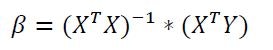
In addition to the above conditions, it is still important to note that the random variable must be distributed according to the normal distribution. Parameter estimates are obtained by the method of least squares.
If a variable X is set for the regression variable (dependent variable) instead of the variable Y, a second regression line is obtained which will coincidence with the Y direction only in case of perfect dependence between variables X and Y. If the regression lines X and Y are close to each other, the relationship between the variables is stronger, and if they form the right angle, the correlation coefficient is equal to zero. If the directions completely match, the connection is functional. Between these extremes, there is a stochastic connection that exists in practice.
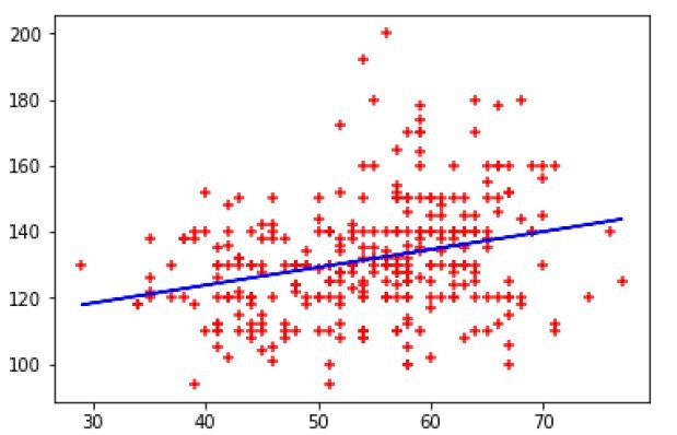
We want to notice the connection between age and blood cholesterol levels or make a predictive linear model that will help us estimate cholesterol levels in a given year. In this case, years are an independent variable, while cholesterol levels are a dependent variable.
```python
import matplotlib.pyplot as plt
from sklearn import linear_model
df = pd.read_csv("heart.csv")
reg = linear_model.LinearRegression()
reg.fit([['age']], tf.trestbps)
The calculated simple linear regression can be graphically represented by the matplotlib library, the X and Y axes are denoted by given variables.
plt.xlabel('blood pressure')
plt.ylabel('age')
plt.scatter(df.age, df.trestbps, color='red', marker='+')
plt.plot(df.age, reg.predict(df[['age']]), color = 'blue')
We get the following graph:
Multiple Linear Regression
The model of multiple linear regression consists of one dependent variable and k independent variables.
The multiple linear regression model is given by the following equation:
Parameter estimates are obtained in a similar manner as for the k-th regression polynomial. The difference is that on the right side of the equation there are several regression variables, not polynomials of one regression variable.
Example calculation of multiple linear regression in Python:
df = pd.read_csv("insurance.csv")
reg = linear_model.LinearRegression()
reg.fit(df[['age', 'bmi']], df.charges)
Graphical representation of more than two regression variables is not easy because it is a so-called hyperplane. In practice, multiple regression is rarely visualized.
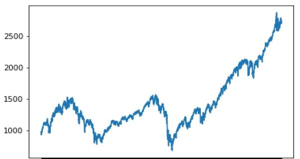
Data Visualization in Python
For data visualization in Python, we use the matplotlib library, which has become the most popular data visualization programming library due to its flexibility and the ability to adjust a large number of parameters.
df1 = pd.read_csv("spx.csv")
df2 = pd.read_csv("heart.csv")

plt.plot(df1.date, df1.close)
plt.xlabel('Date')
plt.ylabel('Price at the close of the stock exchange')
plt.show()
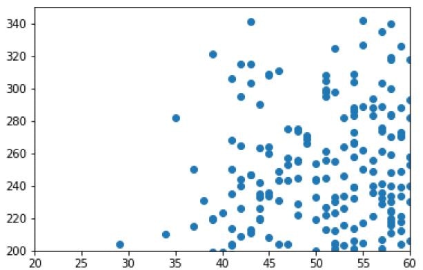
plt.scatter(df2.age, df2.chol)
plt.xlabel('Age')
plt.axis([20, 60, 200, 350])
plt.show()
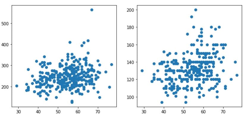
It is possible to show more than one graph at once:
figure = plt.figure(1, figsize=(10, 10))

graph_1 = figure.add_sublot(221)
graph_2 = figure.add_sublot(222)

graph_1.scatter(df2.age, df2.chol)
graph_2.scatter(df2.age, df2.trestbps)
Data Manipulation in Python
Simple Data Manipulation
Simple data manipulation procedures typically involve sorting, filtering, and creating new columns by combining existing data according to some criteria.
df = pd.read_csv('heart.csv')
df.head()

print(df.sort_values('age', ascending = True))
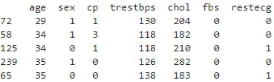
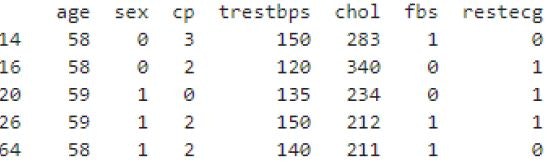
print(df[df['age'].isin(['58', '59', '60'])])
Advanced Data Manipulation
Advanced data manipulation procedures include the criterion of a separate data frame according to the given criteria.
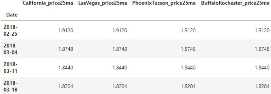
We will calculate moving averages of organic avocados for a period of 25 days for each state separately.
df = pd.read_csv('avocado.csv')
df = df.copy()[df['type'] = 'organic']
df['Date'] = pd.to_datetime(df['Date'])

df.sort_values(by='Date', ascending = True, inplace = True)

new_frame = pd.DataFrame()

for region in df['region'].unique():
   print(region)
   temp_frame = df.copy()[df['region'] == region]
   temp_frame.set_index('Date', inplace = True)
   temp_frame.sort_index(inplace = True)
   temp_frame[f'{region}_price25ma'] = temp_frame['AveragePrice'].rolling(25).mean()

   if new_frame.empty:
      new_frame = temp_frame[[f'{region}_price25ma']]
   else:
      new_frame = new_frame.join(temp_frame[f'{region}_price25ma'])

new_frame.tail()
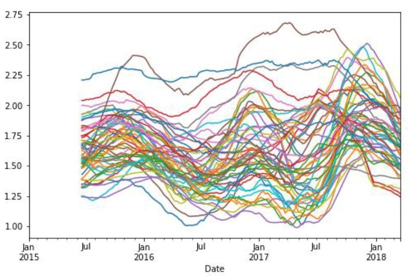
new_frame.plot(figsize=(8,5), legend = False)
The final results of the new frame created according to the given criteria can be seen in the graph below.
Nemanja Grubor
See other articles by Nemanja

WorksHub
Jobs
Locations
Articles
Ground Floor, Verse Building, 18 Brunswick Place, London, N1 6DZ
108 E 16th Street, New York, NY 10003
Subscribe to our newsletter
Join over 111,000 others and get access to exclusive content, job opportunities and more!